In my standard-issue (non-specialist) Digital Technology classes, I’ve attempted to spruce up the Data Representation content in the course.

I found last year, we neglected poor old Data Rep and focussed a little too much on binary conversions – which led to confusion and distress among some students. ¹

For reasons beyond my understanding or pay grade, Digital Technology is now taken one hour a week for the whole year. There are significant downsides to this timetabling ², but one advantage is that the course content divides somewhat neatly into four terms and having five different classes allows me to refine my lessons and activities to a much finer degree than I could last year (with one class at a time).

For first term, I opted to focus solely on a pixel art activity that I have previously (somewhat optimistically) attempted to squeeze into a single lesson.

The activity essentially guides students through creating an image like this:

Through to a numerical representation like this:

20200000000000000000000000000000000000000000000000000
00000000000000000000001100000000000000000101000000000
00000111001100000000000010000000100000000001000000000
10000000010010000000010000001000000000000100000001111
11001000010000000001011011000100000000001001101001000
00000000000001010000000000000000110100000000000000010
01000000000000000001010000000000000000001000000000000
000000000000000000000000000000000

The fast students will get to the stage of writing clear and simple English instructions to read the numbers and recreate the image (as pixel art), but in my 6-7 lessons, I only managed to get the majority of students performing the numerical conversions.

Lesson 1

(The first set of slides can be found here)

It would be remiss of me not to link to the excellent Digital Technologies Hub section on Data Representation in years 7/8.

The flow in DT hub is to cover representation in year 8 only, beginning with binary representation and moving to the way data is encoded and represented numerically.

In addition, my approach to teaching Data Representation is heavily influenced by the CS Unplugged activities collected as Everything is Numbers.

DT Hub’s resources are structured around the ACARA curriculum points which offer tremendous flexibility ³ so there’s no need to follow their suggested progression slavishly.

In WA, our curriculum body has restricted that flexibility somewhat – it is necessary to cover numerical data representation in year 7 before exploring binary representation in year 8.

Truth be told, the content works in any order and there are benefits to either – knowing that data is numbers prior to learning about binary numbers allows for context when it comes to hardware representation of numbers (switches, magnetic polarity etc) ⁴. Doing it in reverse gives a reason for the conversion of data into numbers.

All of this is to simply say that my efforts this time around began with the concept of “thinking” and the idea that computers think of everything as numbers – an attempt to prime students for the relevance of the exercises ahead.

We look at the idea of “abstract representation” – that symbols be a universally understood stand-in for physical objects or concepts (culminating in language itself, numbers etc), using an activity that I shamelessly stole from a PL with James and Bruce.

While this activity (slides 5-12) is not strictly necessary to teach the curriculum, there is value in making clear the fact that the way computers store abstract representations of our data is actually not such a weird concept, it’s something that we humans do too, and in a far less explicit manner.

The activity from slide 13 onwards is the real introduction to the process of converting a “natural” image ⁵ into pixels and ultimately numbers.

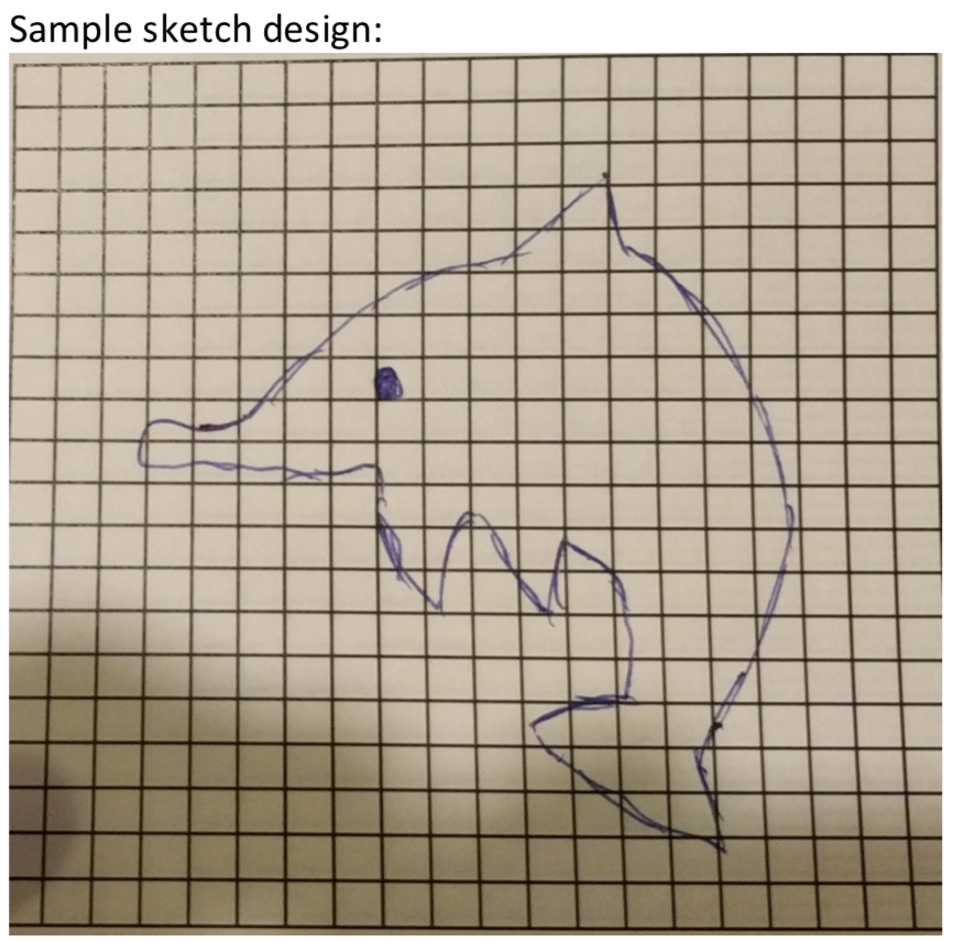
We begin by drawing a simple image of our choosing onto graph paper, ignoring where the grid lines are relative to our drawing⁶. There is an example of a simple picture on slide 15, but I like to draw directly onto the whiteboard with the grid projected to make the process clear.

Students are then to go around squares that encompass the outline of their image and decide, square by square if more than 50% of the square is their picture, or if it is the background. If more than 50% is covered by their picture, they must colour in entire square, if not, the square is left blank.

It is important for students to realise that pixels are an either/or thing (or, in fact, a binary thing) – they may not partially shade a square. If they are unconvinced, have them peer closely at the screens in front of them – there are no half measures with pixels ⁷.

Using the example above, you would end up with something like this:

Natural image converted to “pixels”

Some students are resistant to this stage because:

1. It destructively edits their artwork
2. The resulting blocky thing looks a bit rubbish

That’s good – it makes for excellent discussion fodder. Tell them to push through it.

This brings us to the end of my first lesson on data representation.

In the next lesson, students will look at recreating their hand-drawn representation on screen (and the artistes mentioned above will have an opportunity to improve the pixel version) and then figuring out how to convert that to numbers.

Opportunities for Enrichment & Real World Context

The process by which students take their “natural” image and selectively colour in pixels is akin to the process taking place when a picture is taken in a digital camera.

Photography as a medium is effectively “painting with light” – coloured light enters through a lens and strikes a digital sensor ⁸. The digital sensor has the capacity for a certain number of pixels – usually in the tens of millions as at the time of writing this.

The camera has to make the same kinds of decisions as the students – which pixels to turn wholly one colour or the other.

For our students, the process is slightly simplified as we work in true black and white – only one colour – and we are working with a resolution not much more than 20×20 pixels.

My slides include a representation of the same pixels-on-a-grid image but drawn over pixels half the size (therefore, twice as many pixels or twice the resolution). Students can see that increases in the number of pixels per area of image will result in a more faithful representation of the natural image.

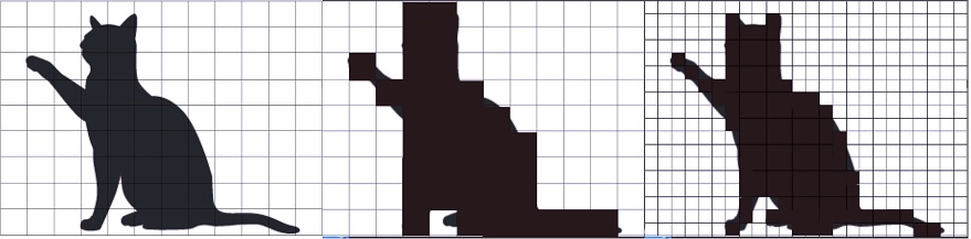
From L-R: A “natural” image, very low resolution, double resolution. Original image is “bleeding” outside the lines to demonstrate the process the students should be following by hand.

Students should also be able to see pretty soon that there are drawbacks to higher resolutions – twice the resolution means twice the number of pixels to “process” and remember, which links very neatly to the reasons why a video game will require more power at a higher resolution or why a better quality photograph will require more space on a hard disk.